Python培训Week6
复习
对数据进行预处理的方式,注意预处理只改变X而不改变y:
- Rescale
- standardlize
- Normalize
- binarize
改进计算准确率accuracy score的方式:
- K-fold
没有考虑到标签分组情况,还不够好 - StratifiedKFold
模型选择思路:
- 均值看准确率
- 标准差看稳定性
更直观的方式:
- 箱子图
- Confusion Matrix 混淆矩阵/模糊矩阵
今天主要有3个专题:
- 将训练好的模型持久化保存
- 从数据预处理到算法评估,搭建一整套框架完整这些任务
- 对数据进行降维处理
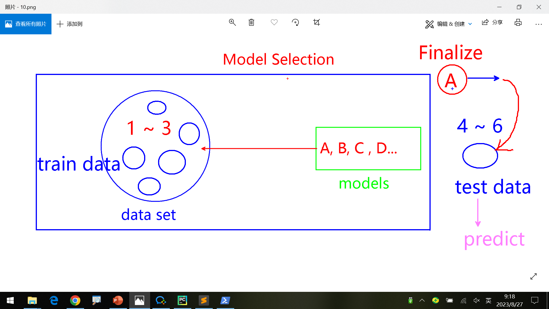
1.Finalize模型固化/持久化
根据数据选择出一个最合适的算法后,将数据、算法参数等存储起来进行Finalize。便于后面用户提供新数据后直接使用。算是Model Selection的Output。
如何保存和使用?
流程是读取数据、使用算法最后训练一次、最后使用pickle将模型(数据和算法)保存。
1 | import pandas as pd |
使用时再读入文件
1 | import pickle |
得到输出
[0]
为什么数据很重要?
单纯软件开发->没有数据积累,客户可以随时更换供应商;
软件开发+数据存储积累->除了软件,还可以根据数据提供相应数据分析报表,增加用户粘性;后期数据越多,数据分析越准确,而且客户要迁移可能还要买回数据,成本很高。
2.Framework(Model Selection)
每次数据分析的流程大致是:
- preprocessing
- model selection
- score
- …
可以将前3步做成pipeline的形式,简化重复劳动
另外还有DataGenerator, 在客户数据到来之前生成模拟数据
1.生成dataset
练习可以用sklearn.datasets的make_*方法,实际一般根据客户真实数据构造
1 | from sklearn.datasets import make_classification |
输出如下:
[[-2.43850005 -0.07321394 0.91037513 … 0.17318305 -0.48545443
0.50529299]
[ 0.26199228 -0.63133888 -0.17787624 … -2.38110847 0.35979645
0.37771326]
[ 0.05085058 0.73357154 0.23160743 … -1.26857873 -2.0520035
0.97842607]
…
[ 0.03034656 0.23028396 -1.90049935 … -0.3695487 -1.75098982
0.13479775]
[-0.1134665 -0.34927547 0.57881782 … 2.05341675 -1.10515843
-1.46092126]
[-0.23639439 -0.4040107 -0.66023956 … 0.59499224 -0.53790146
-0.81610969]]
[1 1 0 0 1 1 1 1 0 0 0 0 1 0 1 0 1 0 1 1 0 1 0 0 1 0 0 0 0 1 1 0 0 0 1 0 0
0 1 1 0 1 0 1 0 0 0 0 1 1 1 0 0 0 0 0 1 0 1 0 1 1 0 0 0 1 0 1 1 0 1 0 0 1
1 0 1 0 0 0 1 1 1 0 1 1 1 0 1 0 1 0 0 1 1 1 1 1 1 0 0 1 0 0 0 1 0 0 1 1 0
0 1 0 1 0 0 1 0 0 1 0 0 1 0 0 0 1 1 1 1 0 1 1 0 0 0 0 0 1 0 0 0 1 1 0 1 0
1 0 1 1 1 0 0 0 1 1 1 1 1 0 1 1 1 0 1 0 0 0 0 0 0 1 0 0 0 1 0 0 0 1 1 0 0
0 0 1 0 0 1 1 1 1 0 1 1 0 1 1 0 1 1 0 0 1 1 0 1 0 1 0 1 1 0 1 1 0 0 1 1 0
1 1 0 0 0 0 1 0 1 1 0 1 0 0 0 0 1 1 0 0 1 1 1 0 1 0 1 0 0 1 0 1 1 1 0 1 0
0 0 1 0 1 1 1 0 1 1 0 0 1 1 1 0 1 0 1 0 0 1 1 1 0 0 1 1 1 0 0 0 0 0 0 0 1
1 0 1 1 1 0 0 1 0 0 0 1 1 1 0 1 0 1 0 1 0 1 0 0 1 0 1 0 0 1 1 0 1 0 0 1 0
1 1 1 0 1 1 0 1 1 1 0 1 1 1 0 0 0 1 1 1 0 0 1 1 0 1 1 1 0 1 0 1 1 0 0 1 0
0 0 1 1 1 0 0 0 0 1 1 0 1 0 0 0 0 1 0 0 0 1 0 1 0 1 1 1 1 0 1 1 0 0 1 0 0
1 0 1 1 0 0 1 0 0 1 1 0 0 0 0 1 0 0 0 0 0 1 0 0 1 0 0 0 0 0 0 1 1 0 0 0 1
1 0 1 0 1 1 0 0 1 0 0 1 0 1 1 0 1 1 0 0 0 1 1 0 1 1 0 0 1 1 1 1 1 1 0 0 1
0 0 1 0 1 0 1 0 1 0 1 0 1 1 0 1 1 1 0 0 1 1 1 0 1 1 1 1 0 0 0 1 0 0 1 0 1
1 0 1 0 0 1 1 0 1 1 1 1 0 1 0 0 1 0 1 0 0 1 0 1 0 0 1 0 0 0 0 0 1 0 0 1 1
0 0 1 0 0 1 1 1 0 0 1 1 1 0 1 0 0 0 0 1 1 1 0 1 1 0 1 0 0 1 0 1 1 1 1 1 1
0 0 1 0 1 1 0 0 0 0 0 0 0 0 1 0 0 0 1 0 1 1 1 1 0 0 0 1 0 1 1 1 1 1 1 1 1
0 0 0 0 1 1 0 1 0 0 1 1 1 0 0 0 1 1 1 1 0 1 0 0 0 0 1 0 1 0 0 1 0 0 1 0 1
1 0 1 1 0 0 0 1 1 1 1 1 1 1 1 1 0 1 1 0 1 1 1 0 1 1 0 1 0 1 0 1 0 1 1 1 0
1 1 0 0 1 1 0 1 1 0 0 1 0 1 1 0 0 1 1 0 1 1 0 0 0 0 0 1 1 0 0 0 1 0 1 0 1
1 0 1 0 1 1 0 0 1 0 0 1 1 0 0 0 1 1 0 1 1 0 1 0 1 1 0 0 1 1 1 0 0 0 1 0 1
0 1 0 0 1 1 1 0 1 0 1 1 0 1 1 1 0 0 1 1 0 1 0 0 1 1 0 0 1 0 1 0 1 0 0 1 1
1 1 0 1 1 0 0 1 0 0 0 0 1 1 1 1 0 1 1 1 1 0 0 1 1 0 0 1 0 0 0 0 1 1 1 1 0
0 1 0 0 0 0 1 1 1 1 1 0 0 0 1 0 0 1 0 0 0 1 1 1 1 1 1 0 1 1 0 1 0 1 1 1 0
1 1 1 0 1 1 0 0 0 0 1 0 0 1 0 0 0 1 0 0 1 0 0 0 0 1 1 1 1 0 0 1 1 1 1 0 1
1 1 1 1 0 0 1 0 0 0 1 0 1 1 0 0 0 1 0 0 0 1 0 0 0 0 0 1 1 1 0 0 0 1 1 1 0
0 0 0 0 1 1 1 0 0 0 0 0 0 0 0 0 1 1 0 0 1 1 0 1 0 1 1 1 1 0 1 1 1 1 0 0 1
1]
2.添加算法
首先需要添加/支持几种算法,这里用之前学过的几种
1 | from sklearn.neighbors import KNeighborsClassifier |
输出:
{‘KNN’: KNeighborsClassifier(), ‘DTC’: DecisionTreeClassifier(), ‘GNB’: GaussianNB(), ‘SVM’: SVC(), ‘LR’: LogisticRegression()}
3.构建Pipeline
一个pipeline是一个处理的完整流程,这里包括标准化,正常化和算法评估。实际生产可以根据需要自定义步骤。
1 | from sklearn.preprocessing import StandardScaler |
对一个算法要执行pipeline中的所有步骤。
因此evaluate_single_model中执行pipeline,进行评估。
1 | from sklearn.model_selection import KFold |
整合
结合之前的代码,得到最后的程序。
首先通过make_classification构建数据;
然后添加所有要评估的算法到字典models中;
接下来写出单个算法评估的流程:构建使用当前算法的pipeline,并使用它执行cross_val_score;
最后遍历models,写出对所有算法进行评估的代码。注意对异常情况的处理等。
最终代码:
1 | from sklearn.datasets import make_classification |
执行结果:
1 | KNN : 0.902 (+/-0.029) |
3.Dimensionality Reduction降维
前面都完成之后,进一步优化。如何在准确度不降低的情况下,如何提高性能?
PCA算法 Principal component analysis
主元分析法,降维是对数据整体做缩放而不是真正把数据减少了,降维后不叫“维(dimension)”叫做“元(component)”
比如原来纬度=8,太小会影响正确率,太大效果不明显,如何确定降维到多少?(feature selection)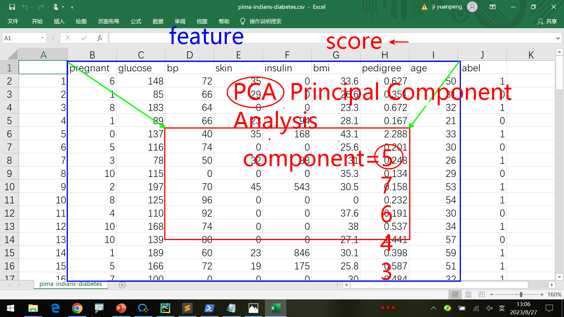
如何降维
可以使用sklearn.decomposition.PCA算法,简单的降维样例如下:
1 | from sklearn.datasets import make_classification |
输出如下
[[ 7.59493044 0.98974276 -12.51113226 11.15523235 -6.955298 ]
[ -9.93846815 4.81754693 -4.11132752 1.45977825 5.09960183]
[ -4.02382826 9.14378059 -0.66566083 8.4283571 -4.53549432]
…
[ -2.4894288 1.14399821 0.79507779 0.23280763 6.41014444]
[-11.87515806 1.99982065 9.13962293 -11.89488371 -4.99407061]
[ 4.43287365 -5.00665058 2.28123668 -2.98325281 5.11717823]]
模型
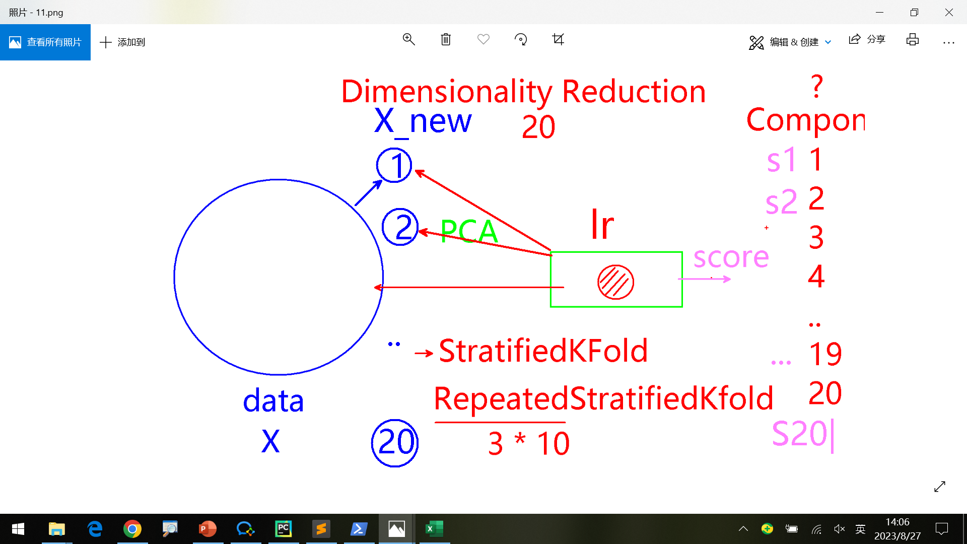
思路
使用同样的算法、对降维后不同纬度的数据计算准确率,从而选出最适合的纬度。
第1次计算数据纬度=1的准确率
第2次计算数据纬度=2的准确率
…
第n次计算数据纬度=n的准确率(相当于没有降维)
准确率计算
之前使用KFold, StratifiedKFold。但这两种在降维方面很难显示出差异,因为各纬度准确度差别很小。
可以使用RepeatedStratifiedKFold(比如每轮10次, 3轮,那么一共是从3*10个数据中得到最后的数据)
以降维到15为例,初步的代码如下:
n_features是属性的总数,n_informative是指有意义的属性的数量,n_redundant是冗余属性的数量。
1 | from sklearn.datasets import make_classification |
输出:
0.8580000000000001 0.03994996871087636
但是模型还不够好,需要人工干预。可以继续优化。
优化
主要修改dimensionality_reduction和define_model,原来这2部分之前需要手动改。
将define_model和dimensionality_reduction结合,修改为返回一个pipeline数组,每个pipeline执行2个步骤,分别是:pca和算法部分。最后修改调用部分,对每个pipeline调用evaluate_model进行评估,并打印数据。
1 | from sklearn.datasets import make_classification |
最后还可以使用boxplot分析数据,更直观地查看各元时的准确率。
如下图,均衡考虑到低维和高准确率,降维到15是最合适的。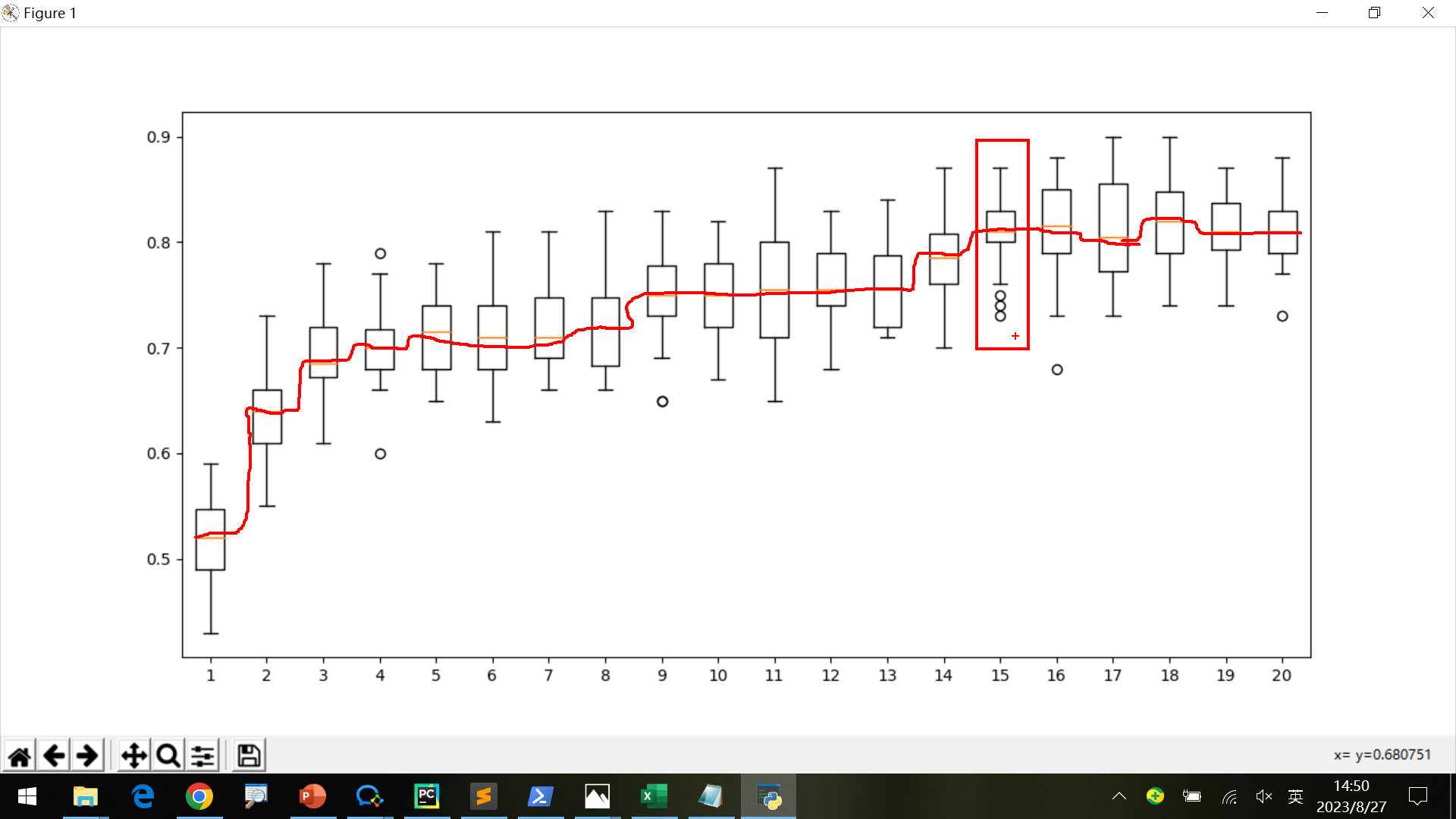
4.frequent item set常用物品组合
使用apriori算法。将数据类似预处理组成新矩阵后,作为算法输入。
1 | from mlxtend.frequent_patterns import apriori |
输出结果:
[‘Apple’, ‘Bananas’, ‘Beer’, ‘Chicken’, ‘Milk’, ‘Rice’]
[[ True False True True False True]
[ True False True False False True]
[ True False True False False False]
[ True True False False False False]
[False False True True True True]
[False False True False True True]
[False False True False True False]
[ True True False False False False]]
support itemsets
0 0.625 (Apple)
1 0.750 (Beer)
2 0.500 (Rice)
3 0.500 (Beer, Rice)
其他
不要拷贝程序
直接拷贝程序学不到东西,还经常需要修改
最好分析思路,再用代码语言写出这种逻辑
读取csv文件列名
像之前糖尿病的csv文件,不是必须写出列名读取。
比如像字母识别的文件,格式如下,可以看出第一列是label,其他是features:
lettr,x-box,y-box,width,high,onpix,x-bar,y-bar,x2bar,y2bar,xybar,x2ybr,xy2br,x-ege,xegvy,y-ege,yegvx
T,2,8,3,5,1,8,13,0,6,6,10,8,0,8,0,8
…
可以按照列名和下标读取:
1 | import pandas as pd |
输出如下:
lettr x-box y-box width high … xy2br x-ege xegvy y-ege yegvx
1 I 5 12 3 7 … 9 2 8 4 10
2 D 4 11 6 8 … 7 3 7 3 9
3 N 7 11 6 6 … 10 6 10 2 8
4 G 2 1 3 1 … 9 1 7 5 10
5 S 4 11 5 8 … 6 0 8 9 7
… … … … … … … … … … … …
19995 D 2 2 3 3 … 4 2 8 3 7
19996 C 7 10 8 8 … 13 2 9 3 7
19997 T 6 9 6 7 … 5 2 12 2 4
19998 S 2 3 4 2 … 8 1 9 5 8
19999 A 4 9 6 6 … 8 2 7 2 8[19999 rows x 17 columns] 0 T
1 I
2 D
3 N
4 G
..
19995 D
19996 C
19997 T
19998 S
19999 A
Name: lettr, Length: 20000, dtype: object
不要做低层次的岗位
一线人员,二线人员……最高层的人员在实验室,平时喝喝咖啡、学习思考,不出面,只做一些思考的工作。
一线的人反而天天各地跑,甚至晚上工作。