复习
Finalize持久化,将算法、参数和数据持久化为一个文件
Framework框架,将模型选择的总体流程打包为一个框架
Dimensionality Reduction降维
frequent item set常用物品组合
今天的内容主要是算法的详细深入讲解,不再是简单调用第三方库,而是完全自己实现用到的算法 ,这才是真正工作中的场景。
Regression Logistic Regression逻辑回归,用于二分的数据,比如判断有/没有患病,有/没有风险。
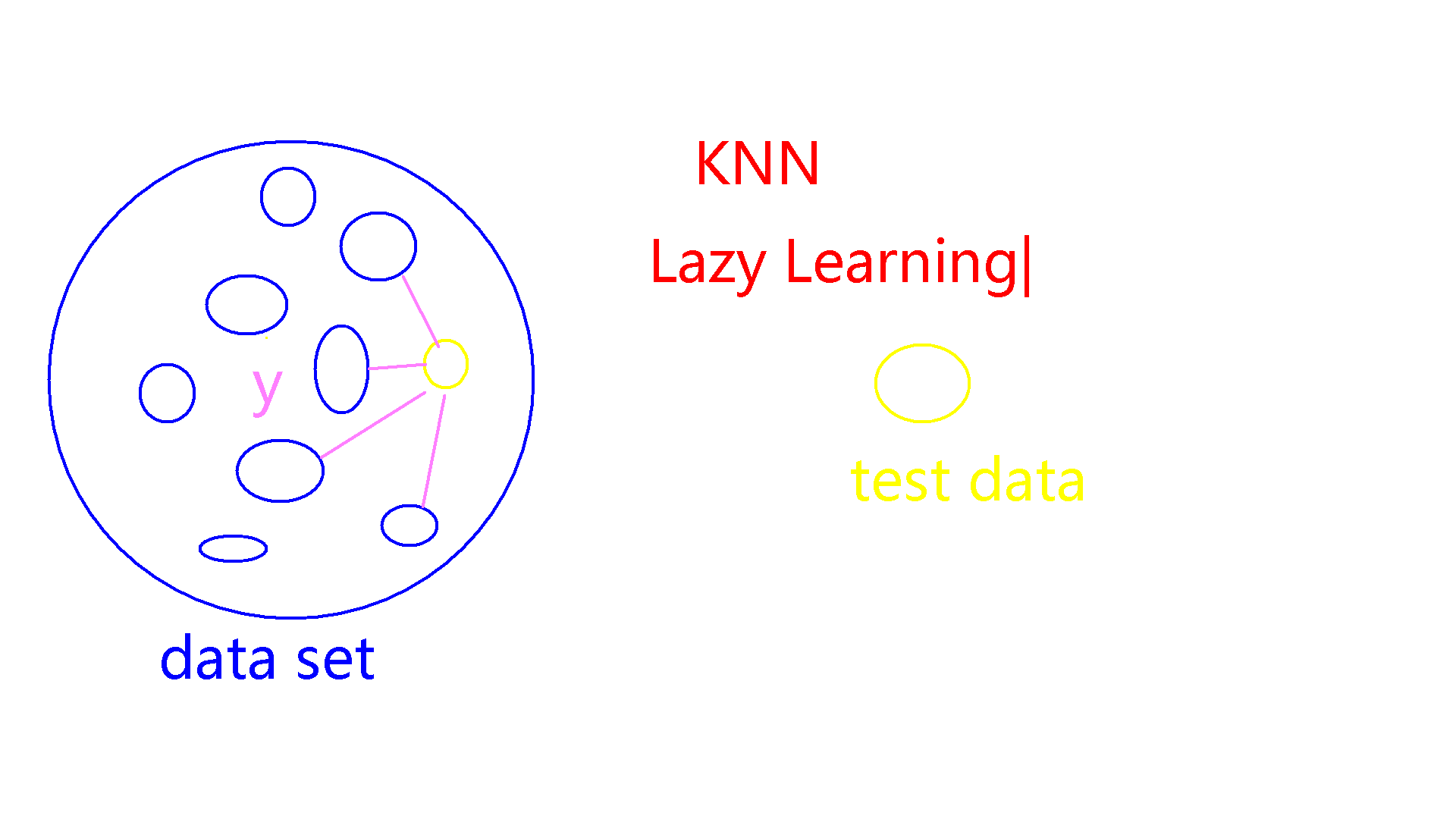
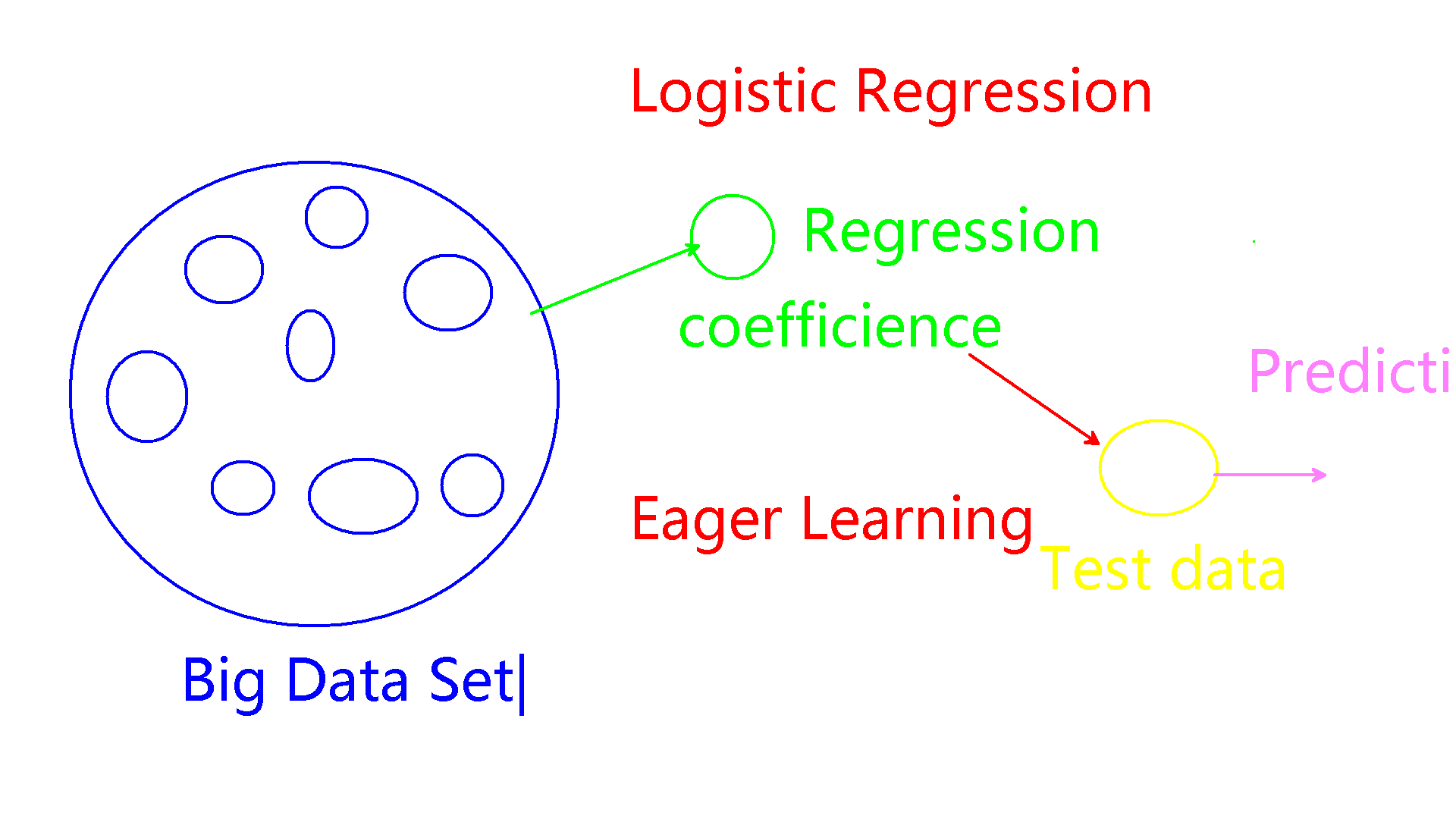
Lazy Learning和Eager Learning 1.KNN算法
2.Logistic Regression
实例 修飞机发动机的老师傅把故障表现存储到数据库中,做成VB程序,让经验不够的徒弟每次遇到问题查询。但这样的方式还不够智能,准确率不够高。最后利用逻辑回归的方式,对每个部件分别评估,得到最终的结果:是否故障(0或1)。这样的工作会替代重复劳动,是大势所趋。算法、人工智能很重要,懂这些知识才不会失业。
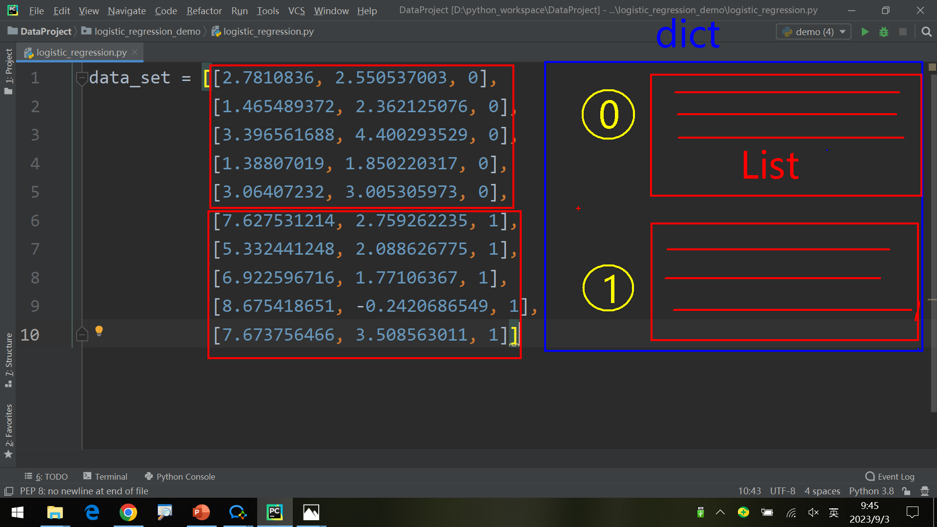
按label分类 如何整理数据,将数据根据label分组?
1
2
3
4
5
6
7
8
9
10
11
12
13
14
15
16
17
18
19
20
21
22
23
24
data_set = [[2.7810836 , 2.550537003 , 0 ], [1.465489372 , 2.362125076 , 0 ], [3.396561688 , 4.400293529 , 0 ], [1.38807019 , 1.850220317 , 0 ], [3.06407232 , 3.005305973 , 0 ], [7.627531214 , 2.759262235 , 1 ], [5.332441248 , 2.088626775 , 1 ], [6.922596716 , 1.77106367 , 1 ], [8.675418651 , -0.2420686549 , 1 ], [7.673756466 , 3.508563011 , 1 ]] def seperate_by_class (data ): seperated_data = dict () for i in range (len (data)): data = data_set[i] label = data[2 ] if label not in seperated_data: seperated_data[label] = [] seperated_data[label].append(data) return seperated_data if __name__ == "__main__" : print (seperate_by_class(data_set))
输出如下:
{0: [[2.7810836, 2.550537003, 0], [1.465489372, 2.362125076, 0], [3.396561688, 4.400293529, 0], [1.38807019, 1.850220317, 0], [3.06407232, 3.005305973, 0]],
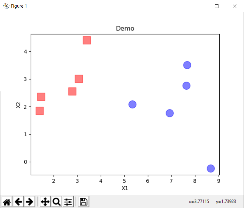
获取各列数据、画图 在上述操作的基础上,还可以获取label分组中第i列的数据,如下:
1
2
3
4
5
if __name__ == "__main__" : seperated_data = seperate_by_class(data_set) data_set0 = [column for column in zip (*seperated_data[0 ])] data_set1 = [column for column in zip (*seperated_data[1 ])]
1
2
3
4
5
6
7
8
9
10
11
12
13
14
15
16
17
18
19
20
21
22
23
24
25
26
27
28
29
30
31
32
33
34
35
36
37
38
39
40
41
42
import matplotlib.pyplot as plt data_set = [[2.7810836 , 2.550537003 , 0 ], [1.465489372 , 2.362125076 , 0 ], [3.396561688 , 4.400293529 , 0 ], [1.38807019 , 1.850220317 , 0 ], [3.06407232 , 3.005305973 , 0 ], [7.627531214 , 2.759262235 , 1 ], [5.332441248 , 2.088626775 , 1 ], [6.922596716 , 1.77106367 , 1 ], [8.675418651 , -0.2420686549 , 1 ], [7.673756466 , 3.508563011 , 1 ]] def seperate_by_class (data ): seperated_data = dict () for i in range (len (data)): data = data_set[i] label = data[2 ] if label not in seperated_data: seperated_data[label] = [] seperated_data[label].append(data) return seperated_data if __name__ == "__main__" : seperated_data = seperate_by_class(data_set) data_set0 = [column for column in zip (*seperated_data[0 ])] data_set1 = [column for column in zip (*seperated_data[1 ])] print (data_set0) print (data_set1) figure = plt.figure() axes = figure.add_subplot() axes.scatter(data_set0[0 ], data_set0[1 ], s=200 , c='red' , marker='s' , alpha=.5 ) axes.scatter(data_set1[0 ], data_set1[1 ], s=200 , c='blue' , alpha=.5 ) plt.title('Demo' ) plt.xlabel('X1' ) plt.ylabel('X2' ) plt.show()
输出图像如下:
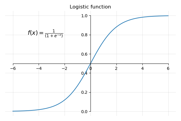
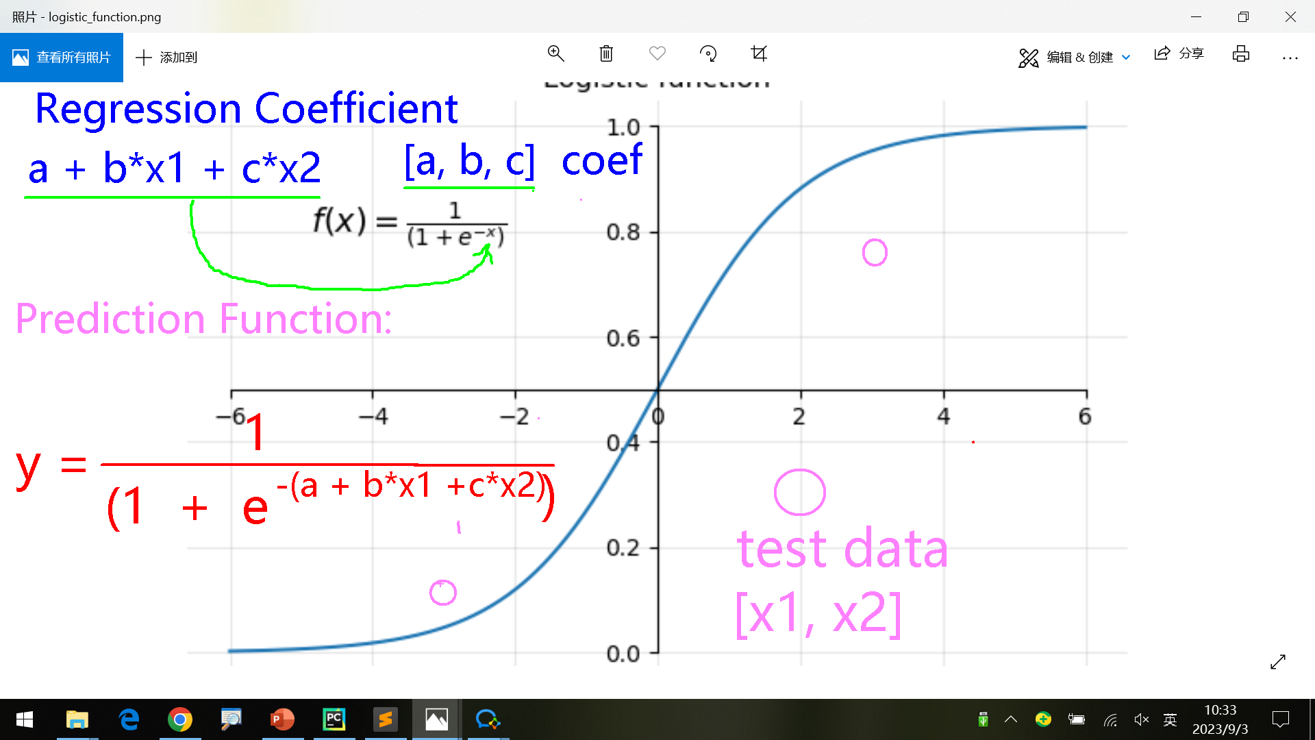
Logistic Regression逻辑回归模型
根据x代入函数f(x)中,得到y在第一象限或者第三象限(取决于y大于0.5还是小于0.5)。
regression coefficient = a+ b * x1 + c * x2
训练后得到的一组常数[a, b, c]就是coef学习算法时,一般会列出最终的公式,往往很复杂。可以反过来,把一个n=1,2,3依次代入,方便理解。
prediction function:
可能采用不同的梯度算法,但是logistic regression模型原理都相同。一般也不用太深入研究算法原理,更多是利用它进行实际应用
大部分算法都是这个难度,少数比这些更难的算法用的频率也很低。
代码实现 主要是把前面的数学公式翻译为代码,比较简单。
1
2
3
4
5
6
7
8
9
10
11
12
13
14
15
16
17
18
19
20
21
22
23
24
25
26
27
28
import numpy as np data_set = [[2.7810836 , 2.550537003 , 0 ], [1.465489372 , 2.362125076 , 0 ], [3.396561688 , 4.400293529 , 0 ], [1.38807019 , 1.850220317 , 0 ], [3.06407232 , 3.005305973 , 0 ], [7.627531214 , 2.759262235 , 1 ], [5.332441248 , 2.088626775 , 1 ], [6.922596716 , 1.77106367 , 1 ], [8.675418651 , -0.2420686549 , 1 ], [7.673756466 , 3.508563011 , 1 ]] def logistic_regression (x ): return 1.0 /( 1 + np.exp(-x)) def predict (test_data, coffiencients ): coef_sum = coffiencients[0 ] for i in range (len (test_data)): coef_sum += coffiencients[i+1 ] * test_data[i] return 1.0 /( 1 + np.exp(-coef_sum)) if __name__ == "__main__" : coef = [-1.6652041168582101 , 2.8997553753773953 , -4.293589516352396 ] test_data = [5.332441248 , 2.088626775 ] y_pred = predict(test_data, coef) print (y_pred)
输出如下:
0.9920756968878671
可以看到,到现在高级阶段就很少用sklearn了,它在行业内做的很好,但是效率等还不够好。实际中往往用它比较少。
这个例子只是展示了如何使用已计算得出的coef来进行计算。实际中还需要计算coef。
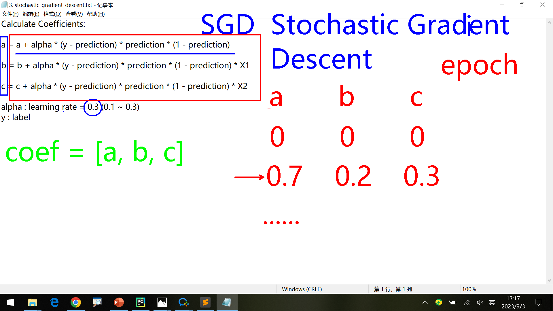
计算coef 1 2 3 4 5 6 7 8 9 10 11 12 13 14 15 16 17 18 19 20 21 22 23 24 25 26 27 28 29 30 31 32 33 34 35 36 37 38 39 40 41 42 import numpy as np data_set = [[2.7810836 , 2.550537003 , 0 ], [1.465489372 , 2.362125076 , 0 ], [3.396561688 , 4.400293529 , 0 ], [1.38807019 , 1.850220317 , 0 ], [3.06407232 , 3.005305973 , 0 ], [7.627531214 , 2.759262235 , 1 ], [5.332441248 , 2.088626775 , 1 ], [6.922596716 , 1.77106367 , 1 ], [8.675418651 , -0.2420686549 , 1 ], [7.673756466 , 3.508563011 , 1 ]] def logistic_regression (x ): return 1.0 /( 1 + np.exp(-x)) def predict (test_data, coffiencients ): coef_sum = coffiencients[0 ] for i in range (len (test_data) - 1 ): return 1.0 /( 1 + np.exp(-coef_sum)) def estimate_coefficients (train_data_set, l_rate, n_epoch ): coef = [0.0 for i in range (len (train_data_set[0 ]))] for epoch in range (n_epoch): sum_error = 0 for row in train_data_set: pred = predict(row, coef) error = row[-1 ] - pred sum_error += error ** 2 coef[0 ] = coef[0 ] + l_rate * error * pred * (1.0 - pred) for i in range (len (row) - 1 ): coef[i + 1 ] = coef[i + 1 ] + l_rate * error * pred * (1.0 - pred) * row[i] print ('Epoch=%d, Learning Rate=%.3f, Error=%.3f' % (epoch, l_rate, sum_error)) return coef if __name__ == "__main__" : l_rate = 0.3 n_epoch = 10000 coef = estimate_coefficients(data_set, l_rate, n_epoch) print (coef)
输出如下,省略了一部分:
Epoch=0, Learning Rate=0.300, Error=2.217
计算coef使用了随机梯度下降(stochastic gradient descent,SGD)算法,另外还有随机梯度上升算法。
a’ = a + …
为了计算[a,b,c]开始默认a=0, b=0, c=0。首先根据第一组数据计算得到新的(a’, b’, c’),然后第二组时,使用上组数据得到的(a’, b’, c’)作为系数,根据第二组数据计算得到新的系数(a’‘, b’’, c’‘),依次类推。
同样的数据,需要多次学习才可以不断提示正确率。因此需要多轮学习(n_epoch很大),使其不断收敛。
数据量很大时,同样计算一万、十万等轮数会非常耗时。生产上,计算中心的云cloud负责计算coef, 用户端只使用这些。
应用 下面是在之前的代码基础上,最简单的样例代码。这里使用了第三方库,还要优化:
1 2 3 4 5 6 7 8 9 10 11 12 13 14 15 16 17 18 19 import pandas as pdfrom logistic_regression_demo.logistic_regression import estimate_coefficientsfrom sklearn.preprocessing import MinMaxScalerfrom logistic_regression_demo.logistic_regression import predictdata_set = pd.read_csv('pima-indians-diabetes.csv' ) mms = MinMaxScaler() data_set_new = mms.fit_transform(data_set) coef = estimate_coefficients(data_set_new, 0.3 , 10000 ) print (coef)test_data = [2 ,1 ,85 ,66 ,29 ,0 ,26.6 ,0.351 ,31 ,0 ] y_pred = predict(test_data, coef) print (y_pred)
首先像实际开发一样,自己实现读取数据的功能。
读取数据 代码如下:
1 2 3 4 5 6 7 8 9 10 11 12 13 14 from csv import readerdef load_data (path ): data_set = [] with open (path, mode='r' , encoding='UTF-8-sig' ) as file: lines = reader(file) for line in lines : if not line: continue data_set.append(line) return data_set data_set = load_data("../pima-indians-diabetes.csv" ) print (data_set)
很多第三方库更新不稳定,可能后面的更新会有很大修改,甚至废弃。这样依赖于第三方库的后期代码维护会困难。
解决方案:
首选自己实现这样的功能。一是避免后期的问题,二是可以完全自定义,比较灵活。
其次如果没有能力,也可以写个wrapper将其包装,代码中全部调用这个wrapper而不是原生第三方接口。后面如果第三方api发生变更或者需要自定义修改,只需要改这一个地方。
但是还有个问题,读取的数字是字符串格式,比如是字符串’12.1’而不是数字12.1。下面进行格式转换。
转换字符串到数字 下面的代码将数据集(输入全部是数据,即不包含表头)转换为数字格式:
1 2 3 4 5 def convert_to_float (data_set ): for data in data_set: for i in range (len (data) - 1 ) : data[i] = float (data[i].strip()) return data_set
注意这个函数的输入只接受数据,不能将表头等不是数字的数据传入 。
转换后的数据(省略部分):
[[1.0, 6.0, 148.0, 72.0, 35.0, 0.0, 33.6, 0.627, 50.0, ‘1’],
下面还需要自己实现对数据的预处理,以代替原来的MinMaxScaler。
预处理 sklearn中的代码写的不错,虽然没有考虑到太多性能、大数据量下的情况等,但是命名规范、算法实现、文档等都可以参考、学习。
查看sklearn的MinMaxScaler()函数注释:
The transformation is given by:
X_std = (X - X.min(axis=0)) / (X.max(axis=0) - X.min(axis=0))
where min, max = feature_range.
其中axis表示行或者列,axis=0表示列,axis=1表示行。缩放分2步:1.计算每列最小最大值、2.计算X_std进行缩放 。
第一部分:计算每列最小最大值
1 2 3 4 5 6 7 8 9 def find_min_max (data_set ): min_max_list = [] for i in range ( len (data_set[0 ] )): col = [data[i] for data in data_set] min_value = min (col) max_value = max (col) min_max_list.append(min_value, max_value) return min_max_list
第二部分:计算X_std进行缩放
1 2 3 4 5 6 def min_max_scaler (data_set, min_max ): for data in data_set: for i in range (len (data) - 1 ): data[i] = (data[i] - min_max[i][0 ]) / (min_max[i][1 ] - min_max[i][0 ]) return data_set
转换后的数据(省略部分):
[[0.0, 0.4, 0.751269035532995, 0.6545454545454545, 0.5833333333333334, 0.0, 0.676056338028169, 0.24016468435498628, 0.7435897435897436, ‘1’],
实际应用分为2步,第一步计算coef,第二步使用它进行预测。
应用:计算coef 1 2 3 4 5 6 7 8 9 10 11 12 13 14 15 16 data_set = convert_to_float(load_data("../pima-indians-diabetes.csv" )[1 :]) min_max_list = find_min_max(data_set) data_set_new = min_max_scaler(data_set, min_max_list) coef = estimate_coefficients(data_set_new, 0.3 , 1000 )
应用:预测 1 2 3 4 5 6 test_data = [2 ,1 ,85 ,66 ,29 ,0 ,26.6 ,0.351 ,31 ,0 ] y_pred = predict(test_data, coef) print (y_pred)
完整代码 logistic_regression2.calc_coef文件:
1 2 3 4 5 6 7 8 9 10 11 12 13 14 15 16 17 18 19 def predict (test_data, coffiencients ): coef_sum = coffiencients[0 ] for i in range (len (test_data) - 1 ): return 1.0 /( 1 + np.exp(-coef_sum)) def estimate_coefficients (train_data_set, l_rate, n_epoch ): coef = [0.0 for i in range (len (train_data_set[0 ]))] for epoch in range (n_epoch): sum_error = 0 for row in train_data_set: pred = predict(row, coef) error = row[-1 ] - pred sum_error += error ** 2 coef[0 ] = coef[0 ] + l_rate * error * pred * (1.0 - pred) for i in range (len (row) - 1 ): coef[i + 1 ] = coef[i + 1 ] + l_rate * error * pred * (1.0 - pred) * row[i] print ('Epoch=%d, Learning Rate=%.3f, Error=%.3f' % (epoch, l_rate, sum_error)) return coef
主要文件:
1 2 3 4 5 6 7 8 9 10 11 12 13 14 15 16 17 18 19 20 21 22 23 24 25 26 27 28 29 30 31 32 33 34 35 36 37 38 39 40 41 42 43 44 45 46 47 48 49 50 51 52 53 54 55 56 57 58 59 60 61 from logistic_regression2.calc_coef import estimate_coefficients from logistic_regression2.calc_coef import predict from csv import reader def load_data (path ): data_set = [] with open (path, mode='r' , encoding='UTF-8-sig' ) as file: lines = reader(file) for line in lines : if not line: continue data_set.append(line) return data_set def convert_to_float (data_set ): for data in data_set: for i in range (len (data) ) : data[i] = float (data[i].strip()) return data_set def find_min_max (data_set ): min_max_list = [] for i in range ( len (data_set[0 ] )): col = [data[i] for data in data_set] min_value = min (col) max_value = max (col) min_max_list.append((min_value, max_value)) return min_max_list def min_max_scaler (data_set, min_max ): for data in data_set: for i in range (len (data) ): data[i] = (data[i] - min_max[i][0 ]) / (min_max[i][1 ] - min_max[i][0 ]) return data_set data_set = convert_to_float(load_data("../pima-indians-diabetes.csv" )[1 :]) min_max_list = find_min_max(data_set) data_set_new = min_max_scaler(data_set, min_max_list) coef = estimate_coefficients(data_set_new, 0.3 , 1000 ) test_data = [2 ,1 ,85 ,66 ,29 ,0 ,26.6 ,0.351 ,31 ,0 ] y_pred = predict(test_data, coef) print (y_pred)
输出如下:
Epoch=0, Learning Rate=0.300, Error=22.999
无监督学习 无监督学习中,数据是没有label列的,需要经过机器学习划分分组、加上label。
customer.txt
1 2 3 4 5 6 7 8 9 10 11 12 13 14 15 16 17 18 19 20 customer1,1.69,0.14,-0.636,0.069,-0.337 customer2,1.69,-0.322,0.852,0.844,-0.554 customer3,1.682,-0.488,-0.211,0.159,-0.1095 customer4,1.534,-0.785,0.002,0.273,-1.149 customer5,0.890,-0.427,-0.636,-0.604,-0.391 customer6,-0.233,-0.691,-0.636,-0.604,-0.391 customer7,-0.497,1.996,-0.707,-0.662,-1.311 customer8,-0.869,-0.268,-0.281,-0.262,3.396 customer9,-1.075,0.025,-0.423,-0.521,0.150 customer10,1.907,-0.884,2.979,2.130,0.366 customer11,0.478,-0.565,0.825,-0.068,-0.662 customer12,0.469,-0.939,0.073,-0.301,3.288 customer13,0.369,0.747,-0.636,-0.626,-0.283 customer14,0.453,1.517,0.073,-0.301,3.288 customer15,0.369,-.747,-0.636,-0.626,-0.283 customer16,0.312,-0.896,0.498,0.954,-0.500 customer17,-0.026,-0.681,0.073,0.325,0.366 customer18,-0.051,2.723,-0.636,-0.749,0.799 customer19,-0.092,2.879,-0.707,-0.734,-0.662 customer20,-0.150,-0.521,1.278,1.392,1.124
代码如下:
1 2 3 4 5 6 7 8 9 10 11 12 13 14 15 16 17 18 19 20 21 22 23 24 from sklearn.cluster import KMeans def load_data (path ): file = open (path, 'r' ) lines = file.readlines() data_set = [] customer_names = [] for line in lines: items = line.strip().split(',' ) customer_names.append(items[0 ]) data_set.append([float (items[i]) for i in range (1 , len (items))]) return data_set, customer_names if __name__ == "__main__" : data_set, customer_names = load_data('./customer.txt' ) labels = kmeans.fit_predict(data_set) print (labels) customer_cluster = [[], [], []] for i in range (len (customer_names)): customer_cluster[labels[i]].append(customer_names[i]) for i in range (len (customer_cluster)): print (customer_cluster[i])
输出如下:
[1 1 1 1 1 1 2 0 2 1 1 0 2 0 1 1 1 2 2 1]
工作相关 未来这种会是1主流。
需要懂编程,同时也懂算法 ,结合在一起才可以,大学的数学知识够用。
这种工作不是培训几个月就可以上手的,一定是前期做过开发、有一定经验,后面慢慢学习、转变等。